

This is the third post in my series where I lay out my favorite interview questions I used to ask at Google until they were leaked and banned. This post is a continuation of the first one, so if you haven’t taken a look yet, I recommend you read it first and come back. If you don’t feel like it, I’ll still do my best to make this post sensible, but I still recommend reading the first one for some background.
Join our discord to discuss these problems with the author and the community!
First, the obligatory disclaimer: while interviewing candidates is one of my professional responsibilities, this blog represents my personal observations, my personal anecdotes, and my personal opinions. Please don’t mistake this for any sort of official statement by or about Google, Alphabet, or any other person or organization.
Apologies for the delay, by the way. In the time since I published the first part of this series, I’ve gone through a number of (very positive) changes in my life, and as a result writing sort of fell by the wayside for a while. I’ll share what I can as things become public.
This post goes way above and beyond what I would expect to see during a job interview. I’ve personally never seen anyone produce this solution, and I only know it exists because my colleague mentioned that the best candidate he had ever seen had blasted through the simpler solutions and spent the rest of the interview trying to develop this one. Even that candidate failed, and I only arrived at this solution after weeks of on-again, off-again pondering. I’m sharing this with you for your curiosity and because I think it’s a cool intersection of mathematics and programming.
With that out of the way, allow me to reintroduce the question:
The Question
Imagine you place a knight chess piece on a phone dial pad. This chess piece moves in an uppercase “L” shape: two steps horizontally followed by one vertically, or one step horizontally then two vertically:
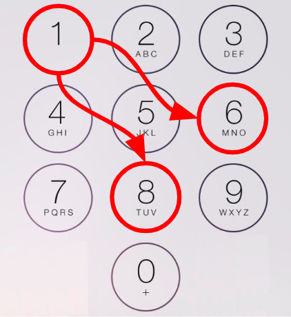
Suppose you dial keys on the keypad using only hops a knight can make. Every time the knight lands on a key, we dial that key and make another hop. The starting position counts as being dialed. How many distinct numbers can you dial in N hops from a particular starting position?
At the end of the previous post, we had developed a solution that solves this problem in linear time (as a function of the number of hops we’d like to make), and requires constant space. This is pretty good. I used to give a “Strong Hire” to candidates who were able to develop and implement the final solution from that post. However, it turns out we can do better if we use a little math…
Adjacency Lists
The crucial insight of the solutions in the previous post involved framing the number pad as a graph in which each key is a node and the knight’s possible next hops from a key are that node’s neighbors:
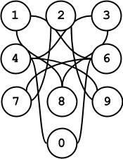
In code, this can be represented as follows:
NEIGHBORS_MAP = {
  0: (4, 6),
  1: (6, 8),
  2: (7, 9),
  3: (4, 8),
  4: (3, 9, 0),
  5: tuple(),  # 5 has no neighbors
  6: (1, 7, 0),
  7: (2, 6),
  8: (1, 3),
  9: (2, 4),
}
This is a fine representation for a number of reasons. First off, it’s compact: we represent only the nodes and edges that exist in the graph (I include number 5 for completeness, but we can remove it without any repercussions). Second off, it’s efficient to access: we can get the set of neighbors in constant time via a map lookup, we can iterate over all neighbors of a particular node in time linear to the number of neighbors by iterating over the result of that lookup. We can also easily modify this structure to determine the existence of an edge in constant time by using a sets instead of tuples.
This data structure is known as an adjacency list, named after the explicit listing of adjacent nodes to represent edges. This representation is by far the most common method of representing graphs, chiefly because of its linear-in-nodes-and-edges space complexity as well as its time-optimal access patterns. Most computer scientists would look at this representation and say “pack it up, that’s about as good as it gets.”
Mathematicians, on the other hand, would not be so happy. Yes, it’s compact and fast to operate on, but mathematicians are (by and large) not in the business of pragmatic ease of use like most computer scientists and engineers. A computer scientist might look at this graph data structure and say “how does this help me design efficient algorithms?” whereas a mathematician might look at it and say “how does this representation allow me to use the rest of my theoretical toolkit?”
With that question in mind, the mathematician might be disappointed by this representation. Personally, this representation of a graph rhymes with nothing I’ve encountered during my mathematical education. It’s useful for writing algorithms, but that’s pretty much it.
Graphs as Matrices
There is another, more fruitful, way to represent a graph, though. You’ll notice a graph is all about relationships between nodes. In the case of an adjacency list, we relate each node with the nodes it’s connected to. Why not instead focus on pairs of nodes? Instead of asking “what nodes are connected to one another with an edge,” you can ask “given a pair of nodes, is there an edge that connects them?”
If this seems like a sort of “six of one, half dozen of another” situation, it is. But the second formulation is magical because it calls into focus something that’s invisible in the adjacency list representation: suddenly we’re very interested in pairs of nodes that don’t have edges. Rather than starting with nodes and computing only the relevant pairs, we start with all possible pairs, and decide whether or not they are relevant later.
We can reframe the adjacency list as follows. Note for each pair (A, B), NEIGHBORS_MAP[A][B] will be 1 if that pair represents an edge in the graph and 0 otherwise:
NEIGHBORS_MAP = {
  0: (0, 0, 0, 0, 1, 0, 1, 0, 0, 0),
  1: (0, 0, 0, 0, 0, 0, 1, 0, 1, 0),
  2: (0, 0, 0, 0, 0, 0, 0, 1, 0, 1),
  3: (0, 0, 0, 1, 0, 0, 0, 0, 1, 0),
  4: (1, 0, 0, 1, 0, 0, 0, 0, 0, 1),
  5: (0, 0, 0, 0, 0, 0, 0, 0, 0, 0),
  6: (1, 1, 0, 0, 0, 0, 0, 1, 0, 0),
  7: (0, 0, 1, 0, 0, 0, 1, 0, 0, 0),
  8: (0, 1, 0, 1, 0, 0, 0, 0, 0 ,0),
  9: (0, 0, 1, 0, 1, 0, 0, 0, 0, 0),
}
Why would we do this? Certainly not to create a more efficient data structure. Our space complexity has gone from being proportional to the number of edges to the number of possible edges, which means N squared, where N is the number of nodes. Iterating over neighbors also just got more expensive: for a given node we get a bunch of irrelevant zeros that we have to filter through.
A mathematician, on the other hand, just got interested. Anyone beyond the junior year of a mathematics undergrad should look at this and immediately say “that’s a matrix!”
(For the sake of brevity, I’ll assume here that you know enough about linear algebra and matrix multiplication to follow along with this post. If you don’t, you can find a great introduction here.)
The wonderful thing about matrices is that they support an algebra. Matrices can be added, subtracted, and multiplied with one another, according to some simple rules. What this particular representation lacks in compactness, it more than makes up for in abstract ease of manipulation.
An Aside
A slight digression: “okay cool”, you might say, “we’ve represented the graph as a matrix. And that matrix can be multiplied by another matrix. What does this have to do with the graph? Who cares?” This is a much more valid question that you may realize, and the answer is “nothing, yet.” Undergrads are my intended audience, so I feel obligated to put you in the right frame of mind before I continue because I’m afraid this might otherwise be more discouraging than enlightening.
After you finish reading this logic presented in the rest of the post, you may be tempted to ask yourself “how the hell was I supposed to come up with that?” I certainly had that reaction time and time again while reading proofs and textbooks. The short answer is: you’re not. At least not immediately. The more proofs and theorems you learn, the more you’ll find you’re able to spot patterns and apply your knowledge. I suggest treating this post as just another tidbit to know and hopefully apply later.
Down to Business
Alright, now that that’s out of the way, let’s get down to the solution. First we’ll explore the structure of this matrix a little. (Note all indices are offsets from zero. This is a departure from mathematical tradition, but this is a CS-oriented post, so let’s go with it.) In this matrix, each row represents the destinations accessible from each key: row 0 has a 1 in position 4 to show you can hop from 0 to 4. It has a 0 in position 9 to show you can’t hop from 0 to 9.
The rows also have a meaning. While the rows represent where you can go from the corresponding position, the columns represent how can get to each position. If you look closely, you’ll notice that the rows and columns look strikingly similar: the i-th position in each row is the same as the i-th position in each column. This is because this graph is undirected: each edge can be traversed in both directions. As a result, the entire matrix can be flipped along its main diagonal and emerge unchanged (the main diagonal is formed by the positions where the row and column numbers are equal).
Now that we’ve introduced representing the graph as a matrix, it’s no longer an algorithmic object but an algebraic one. The particular algebraic operation we’ll be concerned with is matrix-vector multiplication. What happens when we multiply this matrix by a vector? Recall that the formula for multiplying an R row by C column matrix A with an C-length column vector v (short for a matrix with C rows and 1 column) is:
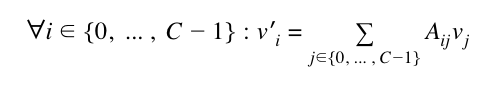
In words, this means that the resulting C-length vector can be computed by taking each row, multiplying each element of that row by the corresponding element in the vector, and adding the component values together. The results are then placed in a vertical, C-by-one matrix, or a C-length vector for short.
This may seem uninteresting at first glance, but that algebraic relation up there is actually the crux of this entire solution. Consider what it means. Each row represents the numbers you can reach from that row’s corresponding key. With this in mind, matrix multiplication is no longer an abstract algebraic operation, it’s a means of summing values corresponding to destinations from a given key on the dialpad.
To make the implications clear, recall the recurrence relation from my previous post:
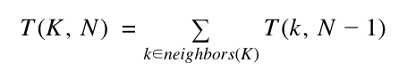
This is nothing more than a weighted sum of values corresponding to destinations from a given key on a dialpad! This framing ignores edges that aren’t in the graph by not even considering them in the iteration, whereas the matrix-oriented one includes them, but only as multiplications by zero that don’t affect the final sum. The two statements are equivalent!
So then what is the meaning of the vector v in all this? So far we’ve been talking almost entirely about the matrix, and we’ve mostly ignored the vector. We can choose any v we want, but we want to choose one that will be meaningful in this calculation. The recurrence relation provides us with a hint: in that case, we start with T(K, 0), which is always 1 because in zero hops we can only dial the starting key. Let’s see what happens with a v where all the entries are 1:

Multiplying the transition matrix by the 1 vector gives us a vector where each element corresponds to the count of numbers that can be dialed in 1 hop. Multiplying again, we can:

Now each element in the resulting vector equals the count of numbers that can be dialed from the corresponding key in 2 hops! We’ve just developed a new linear-time solution to the Knight’s Dialer Problem. In particular:
Logarithmic Time
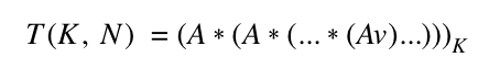
But this solution is still linear. We need to multiply A by the vector v again and again and again, N times. If anything, this solution is actually slower than the dynamic programming solution we developed in the previous post because this one requires unnecessarily multiplying by zero a whole bunch of times.
There is, however, another algebraic property we can use: matrices can be multiplied, and anything that can be multiplied can be exponentiated (to an integer power). Our solution becomes the following:
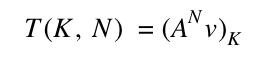
How do we compute A^N? Naturally, one way is to repeatedly multiply A by itself. However, this is somehow even more wasteful than multiplying by the vector: rather than multiplying one vector by A again and again, we multiply all the columns of A again and again. There is a better way: exponentiation by squaring.
As you probably know, every number has a binary representation. If you’ve been studying computer science you already know that this the preferred way of representing a number in hardware. In particular, every number can be represented as a sequence of bits:
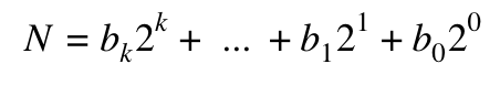
Where k is the largest nonzero bit. For example, 49 in binary is “110001,” or:

Something interesting happens when we perform this expansion for N in our matrix exponentiation solution:
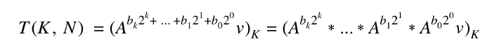
This results in a total of k matrix multiplications. How does k relate to N? k is equal to the number of bits required to represent N, which as you may already know is equal to log2(N). Instead of requiring a number of multiplications that grows linearly in N, we only need a logarithmic number of matrix multiplications! This hinges on a few useful facts:
- A to the power of zero is the identity matrix. Multiplying any matrix by the identity matrix results in the original matrix. As a result, if any bit is zero, we’ll end up multiplying by the identity matrix, and it’ll be as though we ignored it.
- We can compute A to any power of two by squaring the result again and again. A squared is A times A. A to the 4th is A squared times A squared, etc.
This is it! We now have a logarithmic solution.
While this solution requires a little more code than the previous ones on account of the definition of matrix multiplication, it’s still quite compact:
def matrix_multiply(A, B):
    A_rows, A_cols = len(A), len(A[0])
    B_rows, B_cols = len(B), len(B[0])
    result = list(map(lambda i: [0] * B_cols, range(A_rows)))

    for row in range(A_rows):
        for col in range(B_cols):
            for i in range(B_rows):
                result[row][col] += A[row][i] * B[i][col]

    return result

def count_sequences(start_position, num_hops):
    # Start off with a 10x10 identity matrix
    accum = [[1 if i == j else 0 for i in range(10)] for j in range(10)]

    # bin(num_hops) starts with "0b", slice it off with [2:]
    for bit_num, bit in enumerate(reversed(bin(num_hops)[2:])):
        if bit_num == 0:
            import copy
            power_of_2 = copy.deepcopy(NEIGHBORS_MATRIX)
        else:
            power_of_2 = matrix_multiply(power_of_2, power_of_2)

        if bit == '1':
            accum = matrix_multiply(accum, power_of_2)

    return matrix_multiply(accum, [[1]]*10)[start_position][0]
Wrapping Up
On the face of it, this solution seems awesome. It features logarithmic time complexity and constant space complexity. You might think it really doesn’t get any better than that, and for this particular problem you would be right.
However, this matrix exponentiation-based approach has one glaring drawback: we need to represent the entire graph as a (potentially very sparse) matrix. This implies we’ll have to explicitly store a value of every possible pair of nodes, which requires space quadratic in the number of nodes. For a 10-node graph like this one, that isn’t a problem, but for more realistic graphs which might have thousands if not millions of nodes, it becomes hopelessly infeasible.
What’s worse, the matrix multiplication I gave up there is actually cubic in the number of rows (for square matrices). The best-known matrix multiplication algorithms like Strassen or Coppersmith–Winograd have sub-cubic runtimes, but either require extreme memory overhead or feature constant factors that negate the effects for matrices of reasonable size. A cubic-time matrix multiplication starts to become unreasonable with graphs with sizes around the ten thousand range.
At the end of the day, none of these limitations really matter in my mind. Let’s be honest: how often are you going to be computing this on any realistic graph? Feel free to correct me in the comments, but I personally can’t think of any practical application of this algorithm.
The main purpose of this problem is to evaluate candidates on their algorithm design chops and coding skills. If a candidate makes it anywhere near the things I discussed in this post, they’re probably a lot more qualified for the Google SWE job than I am…
If you liked this post, applaud or leave a response! I’m writing this series to educate and inspire people, and nothing makes me feel quite as good as receiving feedback. Also, if this is the sort of stuff you enjoy, and if you’re all the way down here there’s a good chance it is, give me a follow! There’s a lot more where this came from. If you want to ask questions or discuss with like-minded people, join our discord!
Also, you can find runnable the code for this and the previous post here.
Next Steps
After this question was banned I felt like I wanted to start asking a more straightforward programming question. I searched far and wide for a question that was simple to state, had a simple solution, allowed for many levels of followup questions, and had an obvious tie to Google’s products. I found one. If that sounds like something you’d like to read about, stay tuned…
Update: you can check out the rest of the series here: